#pathtozerocarbon, #sustainability
13 – Operational Carbon: Design + Process
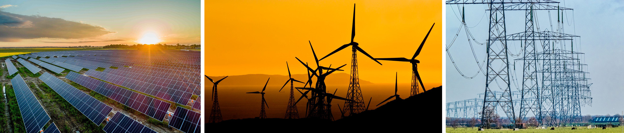
[credit (left to right): Aiseinau [CC BY-SA 4.0], Hernán Piñera [CC BY-SA 2.0], Frans Berkelaar [CC BY 2.0]]
While a major part of greenhouse gas emissions arises from the construction, renovation, and demolition of buildings, the biggest slice of emissions for new buildings—and nearly all from existing buildings—occur during the occupied and operating periods of a building’s lifetime. The primary sources of operational emissions are the fossil fuels used on-site for heating, drying, and/or cooking, and emissions produced by the power plants that generate the electricity used by a building.
Building electrification—avoiding the use of fossil fuels—is the primary operational carbon reduction strategy for buildings, but comes with some calculation complexity since the electricity grid varies in carbon intensity throughout each day and season and is rapidly transforming to use renewable energy. This complexity is the subject of this post, a deeper dive than the companion Post 06.
For a broad, high-level discussion of the electric grid, refer to the earlier Buildings, Energy Use + Carbon post. While we cover many of the same topics, this post focuses on the building level, providing technical details, links, and resources that can help during the design process. Refrigerants are also a significant source of greenhouse gas emissions that do not cleanly fall onto one side of the embodied vs. operational carbon categorization. We consider refrigerant replacement and leaks to also be operational emissions, but they will be covered in the next post, which will focus entirely on MEP systems.
In addition to links in Post 06, useful resources include the U.S. Energy Information Agency (EIA), which provides a wealth of information on U.S. energy production and consumption, at both national and regional levels. Electrification and grid interactivity—from broad overviews to specific, technical discussions—are covered by PG&E’s freely-accessible online courses on a variety of energy-related topics; many of these courses are targeted towards designers and contractors looking to understand and/or implement new technologies and equipment.
On-site Fossil Fuels and Electrification
Once passive design and energy efficiency are implemented, building electrification—avoiding the use of fossil fuels and using only equipment that runs on electricity—is the number one step in reducing operational emissions: the electric grid may currently be “dirty” at some times in some locations, but the grid is becoming cleaner every year, while installing fossil-fuel-based equipment commits buildings to those emissions for decades. For this reason, this post will mostly focus on building emissions from the electric grid.
Heating is the dominant use of fossil fuels in the built environment but is now being replaced with cost-effective electric-based alternatives—mainly the heat pump. Heat pumps are already in use in most buildings to provide cooling; they can simply be run in reverse to provide efficient heat for spaces and hot water. Heat pumps are far more efficient at providing heat than fossil fuel combustion, often providing 2-5 times as much heat as the amount of energy put in (the “coefficient of performance”, or COP), whereas fossil fuel heating equipment is only able to convert 50-95% of the fuel energy into useful heat (equivalent to COPs of 0.5-0.95). Heat pump equipment is now widely available from small residential to large commercial applications.
While heating is the dominant use of fossil fuel in buildings, the other usages are still significant. Clothes dryers have long had electricity-powered alternatives to natural gas versions, but now more energy-efficient heat pump options are becoming more widely available. Diesel backup/emergency generators, which must be regularly run to ensure they are operating properly, and therefore consume fossil fuels every year even when not being used to provide power, can likely be run using (potentially) carbon-neutral biodiesel. The fossil fuel usage with perhaps the greatest reluctance to electrify is for cooking, especially in commercial kitchens. While conventional electric stoves are not as responsive as gas stoves, newer induction stoves provide the quickest response, fastest boiling times, and are far more energy efficient than the other options. They also notably do not contribute to indoor air issues associated with gas that emit unhealthy air pollutants even when turned off. While not yet prevalent, fully-electrified commercial kitchens are starting to become more common, such as at Microsoft’s 77,000 sq.ft. of commercial kitchen at the Redmond main campus redevelopment or Climate Pledge Arena’s all-electric cooking.
Resilience may be raised as an argument to maintain natural gas equipment—”what if the electricity goes out?”—but most natural gas equipment in our buildings requires electricity to run, from the fans in the HVAC systems to the electric starters on the water heaters; natural gas equipment rarely actually provides resilience. On the other hand, full electrification means an entire system of piping and meters can be omitted from a building, leading to some up-front cost savings, while also avoiding the possibility of a gas leak, which occurs in over 100,000 homes each year in the U.S.
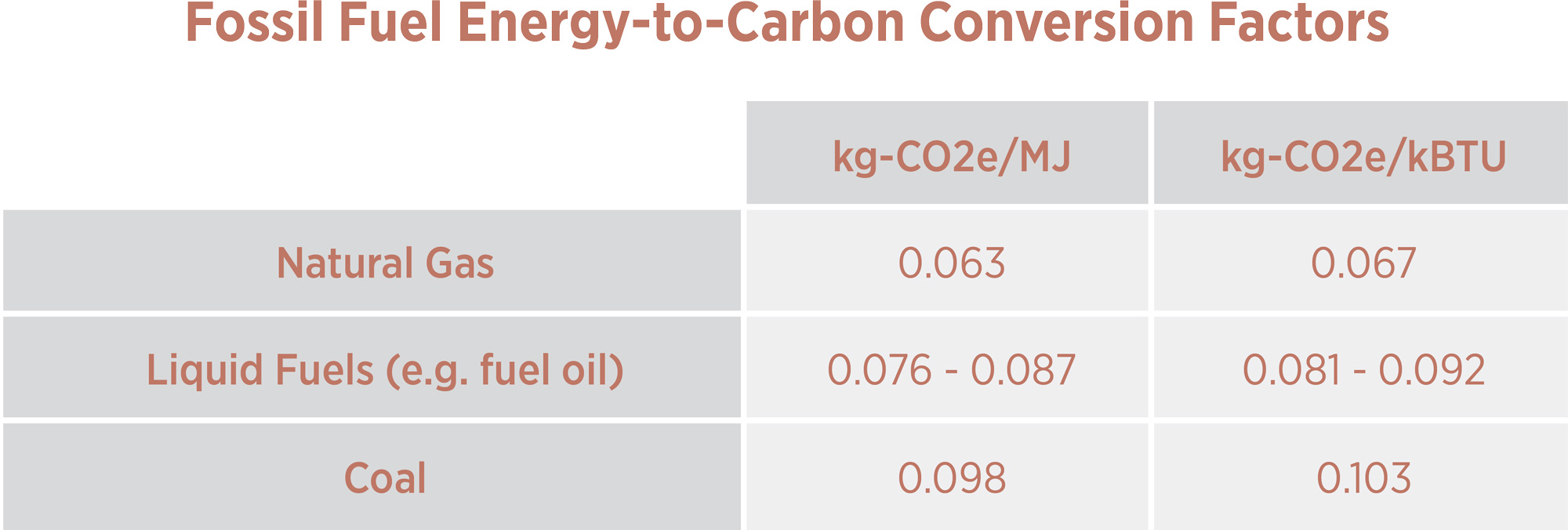
Factors for converting fossil fuel consumption to its corresponding carbon dioxide equivalent (CO2e) emissions over 100 years (GWP100), for energy models that give consumption in terms of energy (J or BTU). These factors include combustion as well as precombustion emissions, which include upstream emissions related to the extraction and transportation of the fossil fuels and methane leakage at wellheads. Conversion factors are from AHRAE Standard 189.1-2020, Addendum m, Table J-11 (see also Table J-6 for more detailed values).
When fossil fuels are used on site and their use is included in energy models—as is often the case for energy models that include mechanical equipment—the corresponding carbon emissions are straightforward to determine: take the amount of fossil fuel used and multiply by the appropriate emission factor, with typical factors shown in the table above. These conversion factors include upstream emissions associated with the extraction and distribution of fossil fuels, which can be significant; the impact of zombie wells, however, are not well understood but contribute to the total carbon footprint of natural gas.
Grid Emissions: Average vs. Marginal
The complexity of how grid carbon emissions are affected by building designs can be seen in the simple example of the grid as illustrated in the below diagrams: 10 identical buildings are provided power by a mixture of renewable (60%) and fossil-fuel-based (40%) power. If each building draws 10 kW of power and the fossil fuel plants generate 1 kg-CO2e/kWh, we can work out that the grid emits 40 kg-CO2e each hour (10 × 10 kW × 40% × 1 kg-CO2e/kWh), with each building accountable for 4 kg-CO2e each hour.
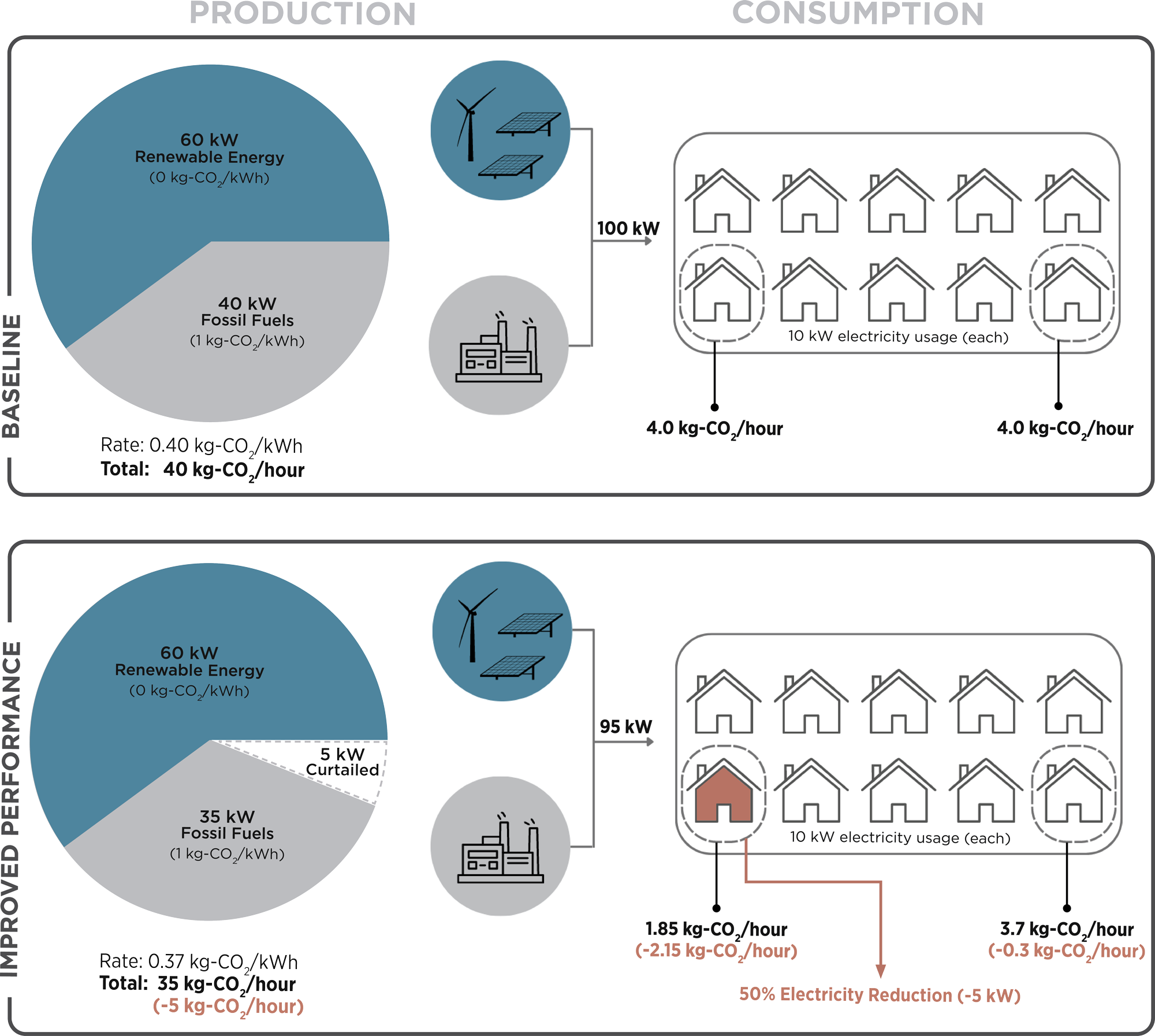
A small grid example, with ten identical buildings drawing from a mix of renewable and fossil fuel generation. The lower panel shows that when one building reduces its electricity consumption by 50%: utilities respond by curtailing (reducing) the fossil fuel power generation, altering the average and total grid emission rate. The energy efficient building reduced its emissions by 2.15 kg-CO2/hr, but the total grid emissions were reduced by a much larger 5 kg-CO2/hr, corresponding to attributional and consequential approaches to understanding design impacts, respectively.
Now we take one of those buildings and reduce the power consumption by 50% to 5 kW; this reduction could be a more energy-efficient alternative to a new construction baseline design, or an energy retrofit of an existing building. When the grid load is reduced, utilities will scale back (“curtail”) output from generators that have quick ramp-up/ramp-down times and are more costly to operate; this is typically fossil-fuel plants—and particularly natural gas plants—as their fuels cost money, whereas renewable energy and nuclear plants cost very little to operate. When curtailing the fossil fuel generation by 5 kW in the example, the energy-efficient building’s grid carbon is reduced to 1.85 kg-CO2e/hr, while the overall grid emissions are reduced to 35 kg-CO2e/hr.
Looking at these numbers more closely, the emissions attributed to the building was reduced by 2.15 kg-CO2e/hr, while the grid emissions were reduced by a much larger 5 kg-CO2e/hr; the former number is the average emissions, while the latter number is the marginal emissions. Where is the difference in the emissions coming from? By causing fossil fuel generation to be curtailed, the energy-efficient design made the grid cleaner: each of the other nine buildings—having done nothing to their electricity usage—have grid carbon attributed to them reduced by 0.3 kg-CO2e/hr. In practice, with millions of buildings on the grid, their attributed emissions would change only by a miniscule amount, but the large difference between the energy-efficient building’s average emissions reduction and the overall grid emissions reduction would remain.
With this example, we illustrated the difference between attributional and consequential approaches to design. Average emission rates can be used to determine the carbon attributed to each building on the grid, all else being equal. However, by evaluating changes in the marginal emissions, designers can determine the actual impact (or consequences) on carbon emissions for a set of energy strategies, which may be far larger or smaller than the impact on attributed (average) emissions. To have the greatest impact on limiting global warming, designers should use marginal emissions when comparing design options and making decisions. That is not to say that average emission rates should never be used: carbon emissions attributed to baseline and/or final designs are still useful metrics. Data on average grid emissions is far easier to come by; in a later section, we discuss sources of marginal emissions data that can be used in building and mechanical design.

When it comes to designing buildings, there is a subtle but important consideration when it comes to marginal emissions: the impact of a new or renovated building on the grid composition and the corresponding effect on carbon emissions. The example above illustrates short-term marginal emissions: how the existing grid responds to instantaneous changes in the demand. When a new building is added to the grid, with new electric loads that will be occurring every day over many years, utilities will respond by creating new generating capacity, such as by installing more PV panels, wind turbines, or perhaps even a new gas plant (when there are enough new buildings to warrant a new power plant of that size). Long-term marginal emissions are marginal emissions that also account for the induced changes in the grid infrastructure by a change in grid loads that occur over many years; it is these long-term marginal emission rates that should be used when it comes to building design. Short-term marginal emissions rates are still useful for e.g. day-to-day operational decisions in a grid-interactive building; see below for a discussion on grid-interactive buildings.
Time-of-Use
The operational carbon intensity of a building varies with time because both the building’s electricity consumption (demand) and the grid generation mix (supply) vary throughout the day and seasons. Because building load curves and grid emission rates can be correlated (higher loads tending to occur when grid emission rates are higher) or anti-correlated (higher loads tending to occur when grid emission rates are lower), a building’s average operational emissions may be higher or lower than its average electricity consumption multiplied by the average grid emission rate. In fact, on an annual basis, using the average electricity consumption and grid emission rates to calculate a building’s operational emissions may differ by as much as 40% from a proper time-of-use analysis; see the below discussion, or this article. This has implications for what “net zero” means: a net zero energy building is not necessarily a net zero (operational) carbon building.
Demand side variations (the building scale). Building load curves are impacted by a variety of things, including:
- Building program: residential, office, school, industrial, etc.
- Season: higher heating loads in the winter or lower school occupancy in the summer, for example.
- Weather: aside from the impact on heating and cooling, cloudy days require more electric lighting, windy days require windows to be closed and increase infiltration, etc.
- Location: in addition to the weather, building codes and common construction materials vary by location.
- Weekend vs. weekday: offices are occupied during the week and empty on weekends, for example.
- Time of day: residential consumption can spike in the early evening as residents return home to cook, watch TV, etc.
- On-site renewables: rooftop PV reduces the amount of electricity drawn from the grid during sunny days.
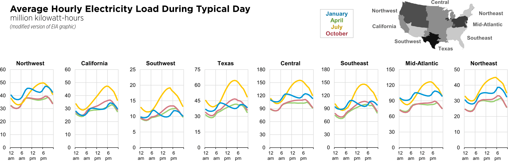
Grid loads vary by region, time of year, and time of day. [credit: modified version of EIA graphic]
Supply side variations (electricity generation and distribution scale). The electric grid carbon emission rates also vary throughout the day and seasons and are affected by many of the same things as in the above (non-exhaustive) list, aside from the building program and on-site renewables. Clean hydro power is more prevalent during rainy seasons or spring melts, but less so during other times of the year. Clean solar power (PV) is more available during long, sunny summer days than short, cloudy winter days. Some power plants are unable to operate at full capacity during extreme cold, extreme heat, or even droughts. The overall grid load impacts the emission rates as high grid loads may necessitate dirty fossil fuel plants be brought online to meet the demand. For these and other reasons, the emission rates can vary rapidly during the course of a day; see this CAISO page for current and historical daily California grid emission curves: the afternoon of Sunday, May 8, 2022 was the first time California achieved 100% renewable energy, but grid emissions spiked only a few hours later as the sun disappeared and renewables were far from capable of meeting the evening demand.
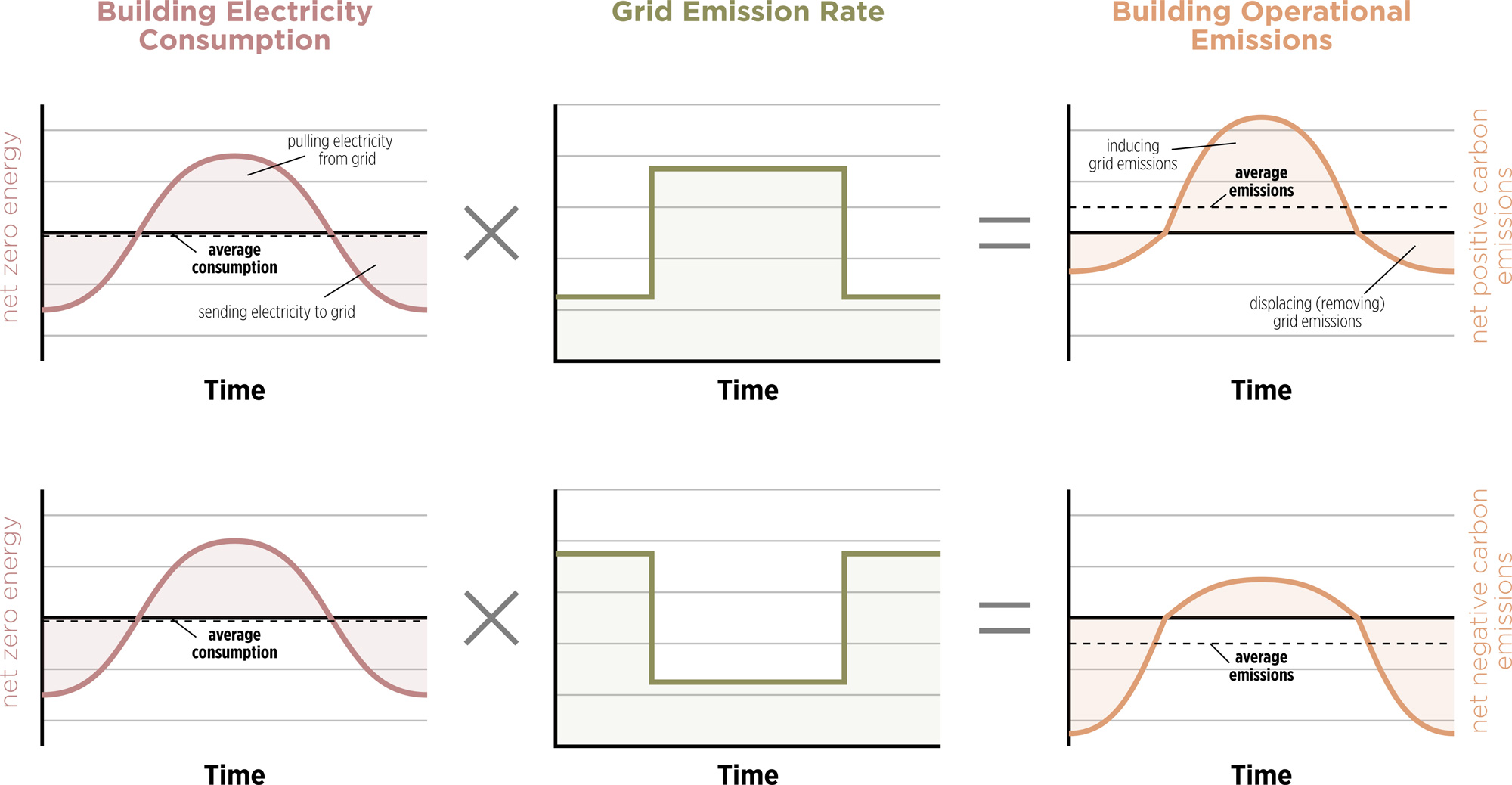
Building operational emissions are the product of the building electricity consumption and the grid emission rate. These two conceptual time-of-use examples show how a building with an average electricity consumption of zero (net zero energy) can have positive average emissions (net positive carbon emissions, top) or negative average emissions (net negative carbon emissions, bottom), depending on how the consumption and grid emission rate curves correlate with each other: net zero energy does not imply net zero carbon emissions.
As time-of-use is important when determining grid emissions, the next two sections will discuss the tools and the process for doing hourly grid emission calculations. For readers more interested in the high-level discussion of operational carbon and not so much the technical details, skip to the Grid Future, Grid-Interactive Buildings, and Electric Vehicles section below.
Grid Carbon Tools
There are many sources of information on the electric grid and corresponding carbon emissions. However, as time-of-use is important in determining the operational carbon footprint, we specifically discuss here tools that allow for local, hourly grid carbon emission analyses.
Cambium. Cambium is an NREL project that simulates the U.S. electric grid down to a local level from the present day through 2050. Datasets include power generation composition (wind, hydro, nuclear, etc.), average emissions, marginal emissions, and various other grid characteristics for each of 48 states (excluding Alaska and Hawaii) or, alternatively, 134 more fine-grained balancing regions. The Scenario Viewer allows datasets to be visualized in a variety of ways, such as generation breakdown in a state over the next 30 years or the hourly marginal emission rates in a region; datasets can also be downloaded from there in CSV format (select “Cambium 2022” or the newest Cambium analysis, then “Download” to get full datasets over all regions). Excel workbooks are also provided for quick, simple analyses, but are currently only available for marginal emissions.
The Cambium project is intended for aiding various groups—such as utilities, government agencies, and the AEC industry—with long-term decision-making involving the U.S. electricity sector. For us in the AEC industry, Cambium provides a free source of local, hourly grid carbon emissions that can be used to estimate the current and future operational carbon in our building designs. Those hourly emissions can optionally include some upstream effects, such as methane leakage due to fossil fuel extraction and processing. While the simulations are performed at hourly timesteps over a full year (8760 hours), datasets are also available at coarser time binning (e.g. monthly averages). If using the Cambium dataset for calculating building operational carbon emissions, be aware that the Cambium year begins on a Sunday and is originally based on 2012 grid and weather data. See the next section (“Calculating Grid Emissions”) for the relevance of these conditions.
Cambium datasets are available for various regulatory and cost scenarios. The “mid-case” scenario factors in only regulations and utility carbon-reduction commitments in place as of the analysis (September 2022 for the Cambium 2022 analysis that is the most recent available as of this article’s publication in 2023), but does not account for any additional regulations and commitments enacted after that year; the mid-case scenario is therefore somewhat conservative, as we expect additional jurisdictions and utilities to make carbon reduction commitments in the future. Other scenarios examined include low- and high-cost renewable energy generation, and achieving 95% carbon reduction by 2050 or 100% reduction by 2035. The 2022 Cambium analyses factor in the renewable energy incentives in the 2022 Inflation Reduction Act; caution should be used when looking at earlier Cambium analysis years as they did not include this important piece of legislation and are therefore much less representative of current conditions. See the documentation for further details on the scenarios available and on how the Cambium analysis is performed.
ASHRAE 189.1-2020 (via Addendum aj) makes use of the Cambium dataset, but to simplify the dataset, they provide a condensed month & hour-of-day binning for use in this standard. See the next section for the impact of coarser time binning on carbon analysis accuracy.
GridOptimal. GridOptimal is a joint USGBC & New Buildings Institute initiative to help with grid interaction and decarbonization, notably developing metrics for evaluating design impacts. A GridOptimal-based pilot credit is available in LEED v4, but even if not pursuing LEED, the freely-available metrics calculator spreadsheet can be used to evaluate and visualize various grid-related performances of both baseline and proposed designs. GridOptimal metrics examine not just the overall operational carbon, but the impact of on-site renewables and demand flexibility, the latter of which can greatly aid utilities in reaching their own carbon reduction commitments. GridOptimal currently uses Cambium data for some of their tools, including the metrics spreadsheet.
WattTime. WattTime is a non-profit program that provides recent (since about 2019), current, and predicted local grid marginal emissions at an hourly or sub-hourly level. Data is accessible through a web API, making it easy to integrate into new tools and workflows. While the other tools mentioned in this section are useful for evaluating proposed building designs, WattTime’s emission forecasts (up to 72 hours) can be used in real-time by building systems to reduce or shift loads during high carbon intensity periods, such as dimming lighting or pre-heating a domestic hot water tank. In other words, the forecasted data can be used to implement the demand flexibility that lowers a building’s operational carbon and helps utilities when most need. Access to most WattTime data requires a paid subscription, but a free account can be used for testing their service.
Electricity Maps. Like WattTime, this commercial service provides historical, current, and predicted (up to 24 hours) local grid emissions data at the hourly level. Unlike the other tools discussed so far, which focus mainly on the U.S. and possibly Canada, this service provides data for many areas around the world, including much of Europe, South America, and Australia. A web API is also available for accessing data, and some basic information can be explored through their online app.
Calculating Grid Emissions
This section provides a condensed description of calculating hourly grid emissions for energy models and some caveats.
For any project that runs energy models, calculating the associated grid carbon emissions is actually a simple and straightforward process, often taking only 5-15 minutes: take the hourly electricity usage from an annual energy model run (an “8760” file), grab the hourly grid emission rates for the project’s location from Cambium or one of the other grid tools previously discussed, multiply them together hour-by-hour (using Excel, Pandas, or any data analysis tool you prefer), and add the hourly carbon numbers up to get the annual grid carbon emissions; a unit conversion may be necessary (see technical details below). Only the net electricity consumption should be considered: subtract any on-site renewable energy and use only the electricity drawn from (or exported to) the grid. For energy models that incorporate natural gas usage, the hourly gas consumption can also be summed, then multiplied by 0.063 kg-CO2e/MJ (0.067 kg-CO2e/kBTU) to get the annual gas carbon emissions.
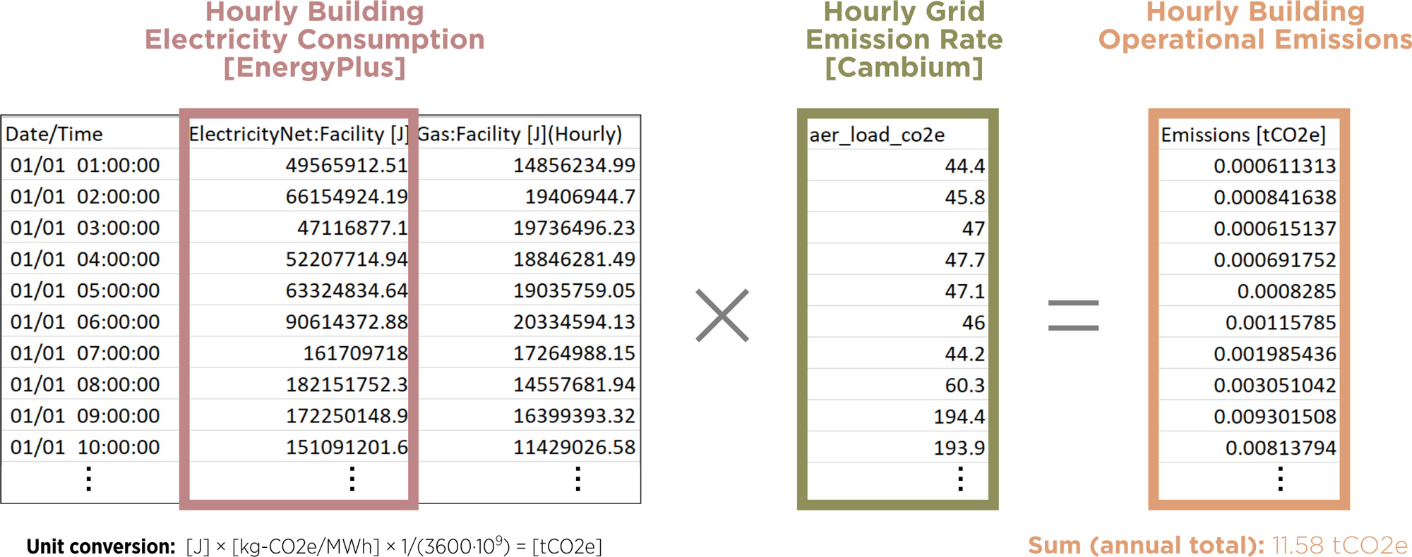
Grid carbon emissions estimates from energy model results in under 10 minutes: take the 8760 (hourly) energy model electricity consumption data, multiply by the local Cambium hourly grid emissions, and apply a unit conversion factor to get the hourly operational emissions; sum the resulting hourly emissions data to get the annual emissions. If included in the energy model, natural gas usage can also be summed and a conversion factor applied–see previous conversion factor table–to get the other major contribution to operational carbon emissions. District energy systems require more specific carbon factors.
Particularly when it comes to simple energy modeling tools aimed at architects, hourly electricity usage is not always provided. The process above can also be applied to any coarser, non-hourly time bins that are available, such as monthly or even just the annual electricity consumption. However, as time-of-use is important, coarser time binnings can produce much less accurate grid carbon estimates, with monthly (12) and annual (1) binning differing from the more accurate hourly binning estimates by as much as 40%. Binning by hour-of-day (24) or month & hour-of-day (12×24) is better (off by up to 8%), but binning also by weekday and weekend separately (2×12×24) yields results almost as accurate as a full hourly analysis (within 1-2%). The high accuracy of the last binning case has a surprising implication: day-to-day fluctuations in the weather have an almost negligible impact on the accuracy of annual operational carbon estimates.
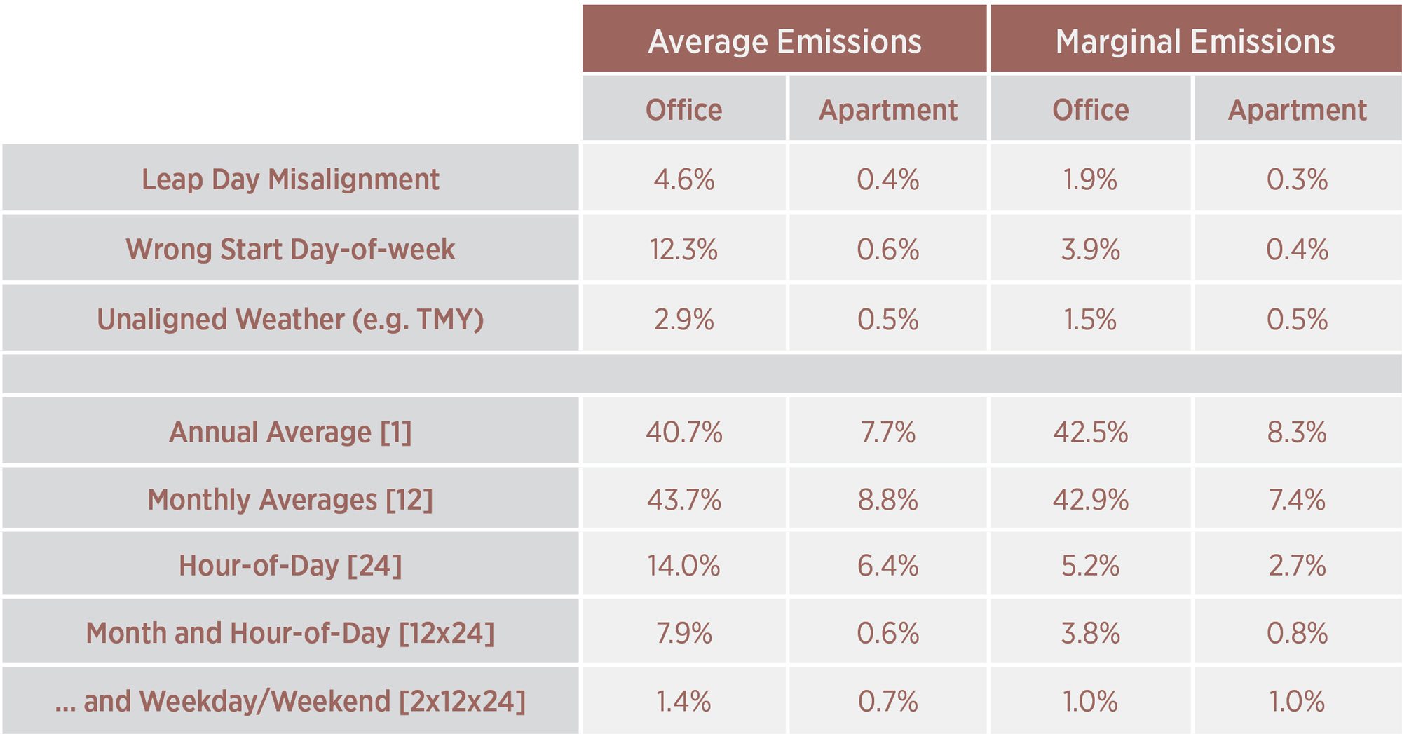
Maximum deviation of carbon emission estimates from a proper hourly, weather-aligned emissions analysis under different energy model / grid emissions data alignments and time binnings. The analysis uses the medium office and mid-rise apartment DOE/PNNL prototype building models from eight cities in the U.S., along with the NREL Cambium 2021 grid emissions dataset (all modeled years). The numbers here represent the level of inaccuracy that can be expected if not doing a full hourly carbon emission analysis, although these are worst case deviations, with many cases of building program & location combinations exhibiting lower levels of inaccuracy.
One might expect that day-to-day weather is important to both the hourly building loads and hourly grid emission rates: during very hot weather, for example, a building draws extra power to run the air conditioning and, because the same is true of nearly all the buildings on the grid, the grid emissions can become worse as the utilities bring on dispatchable fossil fuel plants to meet the high demand. While this correlation can be important at the hourly level, it has a relatively small impact when aggregating emissions over a full year: if running an energy model using weather data that does not align with the weather that occurred during the grid emission rate determinations, the annual emissions will be off by at most 1-3% relative to a proper weather-aligned analysis. This may be due to weather fluctuations being only a small part of the total variations, or e.g. that grid emissions on a very hot California summer evening are not altogether that much worse than on a merely hot California summer evening. In any case, the upshot is that the readily-available TMY weather files that designers so often use for building simulations can be reasonably used in place of actual weather data that corresponds to the grid emissions (Cambium is based on 2012 weather and grid data).
Technical details. When drawing from Cambium datasets, use the aer_load_co2e and lrmer_co2e columns for average and marginal grid emission rates, respectively. For EnergyPlus users, hourly net electricity and gas usage can be exported by adding the following to the IDF file:
Output:Meter:MeterFileOnly,ElectricityNet:Facility,Hourly;
Output:Meter:MeterFileOnly,Gas:Facility,Hourly;
Weekday alignment of the Cambium and energy model data is important: Cambium data begins on a Sunday, so if the energy simulation does not begin on a Sunday, either hourly dataset should be rotated by a few days (e.g. move the last two days of the Cambium data to the beginning) to bring the weekdays into alignment. For energy consumption in J and grid emission rates in kg-CO2e/MWh, like EnergyPlus and Cambium data respectively, multiply by an extra factor of 1/(3600·109) to get the final emissions in tCO2e.
Grid Future, Grid-Interactive Buildings, and Electric Vehicles
The grid is becoming cleaner, with over 60% of the U.S market currently committed to achieving 90% or higher carbon-free electricity production by 2050 and this number is increasing. However, since buildings demand a majority of electricity and electric vehicles (EVs) will also become a major draw on the grid, the utilities will need a lot of help from the AEC and transportation sectors to reach and expand those targets.
Renewable solar and wind energy generation are now cheaper than most other sources of power—including fossil fuels—with costs continuing to decrease. They also have no operational fuel costs. However, solar and wind power are intermittent: they produce power when the sun and wind are available, not necessarily when the power is needed by the end user. To avoid the use of dispatchable fossil fuel plants—which can be ramped up and down to fill in the gap between the grid load and the baseline + intermittent renewable production—the grid will require a combination of energy storage, load shedding, and load shifting. Utility-scale energy storage is a practical way to make intermittent energy generation more dispatchable, but current storage technologies are relatively expensive, with levelized costs far exceeding that of a natural gas plant in most cases, although storage is closer to cost-competitive for peaker power plants that mainly sit idle. The cheapest option is to rely on building-scale load shedding and load shifting, to flip the energy production vs. consumption priority: instead of altering the electricity production to meet the grid loads, what if we alter the loads to better match the renewable energy grid production? By designing towards the grid and using systems that dynamically respond to the grid conditions, we reduce the cost for utilities—and consumers—to build out a clean grid.
Designers have many ways to better work with the grid, ranging from passive design elements to automated, interactive systems. On-site batteries can store excess on-site PV power until it is needed, or can simply be charged using off-peak (lower cost) grid power; the resilience they can provide during power outages are another benefit. Thermal storage and geothermal systems are great ways to reduce peak heating and cooling power draws because the heat or coolth does not need to be generated right when it is used. Passive shading elements, low-SHGC glazing, and/or electrochromic glazing can also reduce peak solar loads, which are a major contributor to peak cooling needs. Demand-response (load shedding) systems can act in response to utilities requests for lowering power use: while large industrial customers might shut down for a few hours during these demand-response events, most commercial and residential responses would have only modest impacts that do not prevent normal occupant usages from occurring, such as reducing lighting by 25% or adjusting thermostat setpoints by a few degrees. Some loads can be shifted away from times of grid stress, such as heating the water stored in hot water tanks: these tanks rarely need to be refilled immediately after use, and some of their capacity can wait to be refilled until energy is more readily available either locally (on-site PV) or on the grid. California’s recently adopted JA13 appendix to their energy code pushes builders to use smart heat pump water heaters that work interactively with the grid to reduce their grid impact, while continuing to provide hot water at the times and capacities they are typically needed in the home; the NRDC, water heater manufacturers, and other stakeholders worked to develop this code and ensure products were readily available on the market. These are only a few ways for designers improve their buildings’ impact on the grid; there are many more possibilities, with the local utility’s website often a source of useful information. Some utilities even provide free design consultation to design teams. Utility incentives and rate structures—particularly rates that vary by time of use and capacity (peak usage) charges—mean any extra up-front costs in using more grid-friendly systems can be partially or fully offset in the long run.
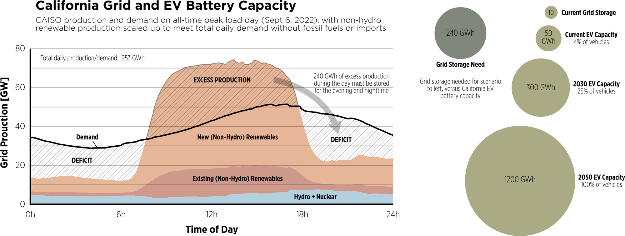
(left) California’s grid demand over the all-time peak load day (September 6, 2022). Also shown is the renewable generation that day scaled up to match the total daily demand (953 GWh) without the use of fossil fuels or imports. In this scenario, 240 GWh of excess production during the daytime, primarily from solar power, would need to be stored for use in the evening and nighttime. (right) The grid storage needed for this extreme load case compared to the storage capacity of electric vehicles (EVs) in California. In the future, use of grid-connected EVs for temporary energy storage can help utilities reconcile the difference between the grid production and load curves. Graphic based on data from CAISO and EVAdoption.
Grid-interactive design options are also discussed in Post 06, but now we turn to a topic we have not focused much on before: EVs, their interaction with the grid, and how they relate to our buildings. Transportation is a huge contributor to our carbon footprint: vehicles that come and go from buildings are typically treated as independent of those buildings when it comes to energy and environmental footprints. This is changing as vehicles become electrified, with EV charging occurring through buildings’ electrical systems; transportation energy is now part of the electrical sizing and design of buildings, and buildings are potentially becoming accountable for vehicle energy consumption. While the AEC and our clients can promote EV adoption by simply providing charging infrastructure—an environmental win in and of itself—there are big opportunities to make the EV charging interactive with the grid in ways that are beneficial to both the utilities and the EV owners.
The first opportunity is the use of smart charging systems to reduce or halt charging during periods of grid stress. Most daily EV usage does not require the battery to be fully charged: just like a gas tank that is 2⁄3 full doesn’t cause stress, a partial battery charge is often enough for several days of commuting and/or running errands, so delaying charging by a few hours or a day has minimal impact on the EV user. Unlike internal combustion vehicles which require a dedicated trip to a gas station to refuel, EVs usually have ample opportunities to charge at home, at work, or even at the grocery store, so later opportunities to charge are easy to come by and, with nationwide rollouts now in progress, will get much more convenient. Utilities and even building owners can incentivize charging during certain non-peak periods through time-of-use charges (whether fixed or dynamically changing) whereby it is cheaper to charge an EV when the grid has a lower-carbon, higher renewable fraction. Smart charging systems can help automate the process.
The second EV grid-interactivity opportunity is for EVs to provide power to the grid. Parked EVs are essentially underutilized batteries, sitting idle throughout the day, storing energy that can be temporarily sent to the building and/or grid when power is most needed. Smart systems would limit how much power is sent to the grid so that the EV owner maintains sufficient charge to use the vehicle. Such systems would require opt-in by the EV owner, but would be to their benefit: the utilities or building owner would pay the EV owners for their power, at a premium that would more than cover the cost of recharging the battery later. Utilities would pay premium rates because it allows them to avoid the high capital costs of peaker plants or their own (expensive) utility-scale battery systems. This scenario is a win-win for utilities and EV owners, but is not yet a common practice.
Conclusions
While using electricity is clearly a long-term, low-carbon strategy, calculating the associated carbon emissions is complex. Forward-looking carbon data projections from electricity should be used during building design to compare options since the grid is rapidly increasing the share of renewable energy. Once buildings are completed and occupied, building owners can use short-term projections to activate grid-interactive technologies to lower carbon emissions and energy costs. While architects do not need to understand grid operations completely, talking with building owners and energy analysts about carbon requires a minimum level of familiarity with topics as covered in this post. We expect the industry to adopt clear practices to account for electricity-related carbon over the next few years and submit this write-up as part of the effort. Some software is already including these hourly emissions.
Thanks to our external collaborators and peer reviewers
Jamy Bacchus (ME Engineers), Greg Collins (Zero Envy), Pieter Gagnon (NREL), Henry Richardson (WattTime), Jack Rusk (EHDD), Forest Tanier-Gesner (PAE Engineers), Jesse Walton (Mahlum), Caroline Traube (McKinstry), Matthew Veloz (FSI Engineers)
LMN Architects Team
Huma Timurbanga, Justin Schwartzhoff, Jenn Chen, Chris Savage, Kjell Anderson
Posted: 06/08/2023
Edited: 09/25/2023
The text, images and graphics published here should be credited to LMN Architects unless stated otherwise. Permission to distribute, remix, adapt, and build upon the material in any medium or format for noncommercial purposes is granted as long as attribution is given to LMN Architects.